An acquisition decision, why two identical buildings don't deserve the same bid
A rent-controlled building comes across your desk. The numbers look solid:
- 100 units
- Market rent averages $2,000/month
- In-place rent averages $1,800/month
- 10% embedded rent
In your experience, similar properties have an average turnover of 20%, so your underwriting model shows that 10% upside unlocking over your 5-year hold. Cap rate compression gives you a nice exit. The IRR clears your hurdle.
You're ready to bid.
But here's the question traditional models can't answer: Will that 10% embedded rent actually materialize within your hold period?
The simple math (and what it assumes)
Most acquisition models handle embedded rent like this:
- Apply a uniform turnover rate (say, 20% annually)
- Each year, 20% of units reset to market
- Embedded rent unlocks in a smooth, predictable pattern
- Value compounds steadily through your hold period
The math is clean and the model is tidy. The problem is what this approach quietly assumes about tenant behavior.
What 20% turnover really means
A 20% annual turnover rate implies the average tenant stays 60 months. But averages hide critical variance.
Here's what gets uncomfortable: if you compound these odds, year after year, over a longer period of time, the odds of a tenant staying in their unit becomes very low. With 20% uniform turnover, in effect your model is saying:
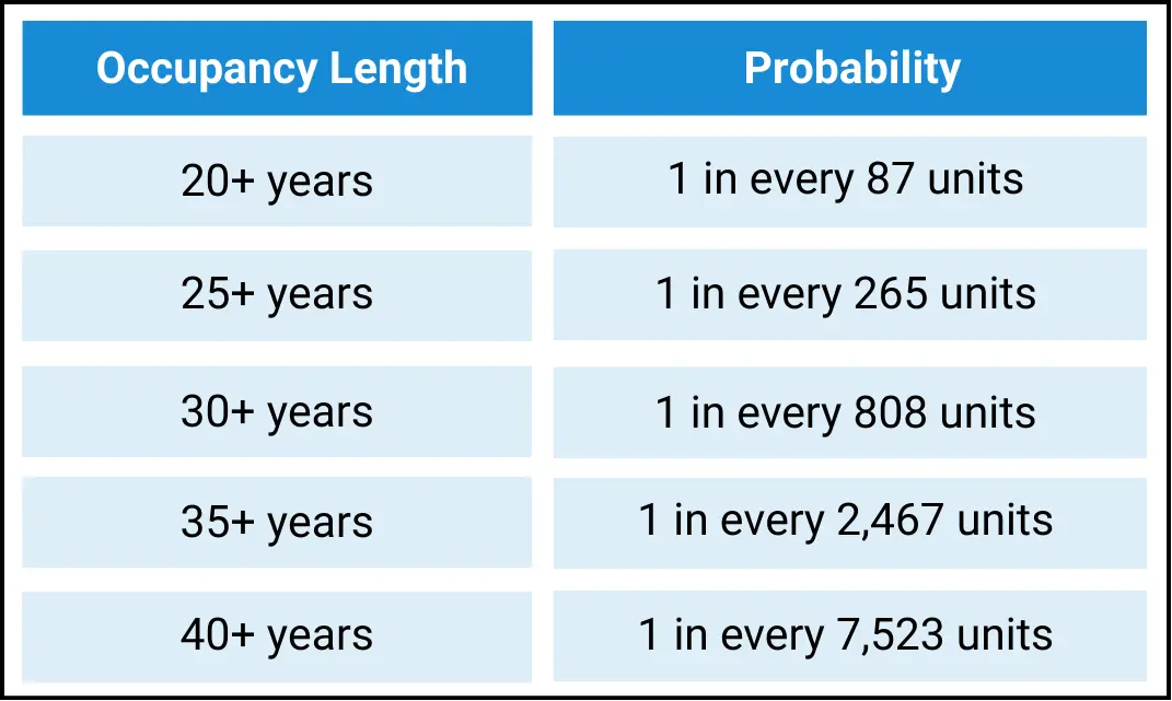
Now think about your actual portfolio. How many long-term tenants do you have? If those numbers are higher than the table suggests—and they almost certainly are—your uniform turnover assumption is wrong. The model is claiming these outcomes are rare statistical events when they're actually common.
The reason: tenants don't behave uniformly. Some are extremely likely to stay (those with deep discounts). Others are likely to leave (those at or above market). Your model treats them identically.
That assumption breaks down completely in rent-controlled buildings because you are operating in a locked-in real estate system.
The tenant behavior you're not seeing
Consider two tenants in your building:
Tenant A is paying $1,950—just 2.5% below market. If rents stay flat or decline, they have little reason to stay. If a competitor offers a deal, they'll move. If they get frustrated with anything, there's no financial penalty to leaving. Your model says they'll stay 5 years. Reality? Maybe 30 months.
Tenant B is paying $1,600—20% below market. They're saving $400/month versus moving. That's $4,800/year. Every year they stay, their discount compounds. Their discount could be so large that even downsizing will cost them more money. They're extremely unlikely to give that up voluntarily. Your model also says they'll stay 5 years. Reality? Maybe 8+ years.
Your underwriting treats them identically. But they're playing completely different games.
Counting cards in rent control
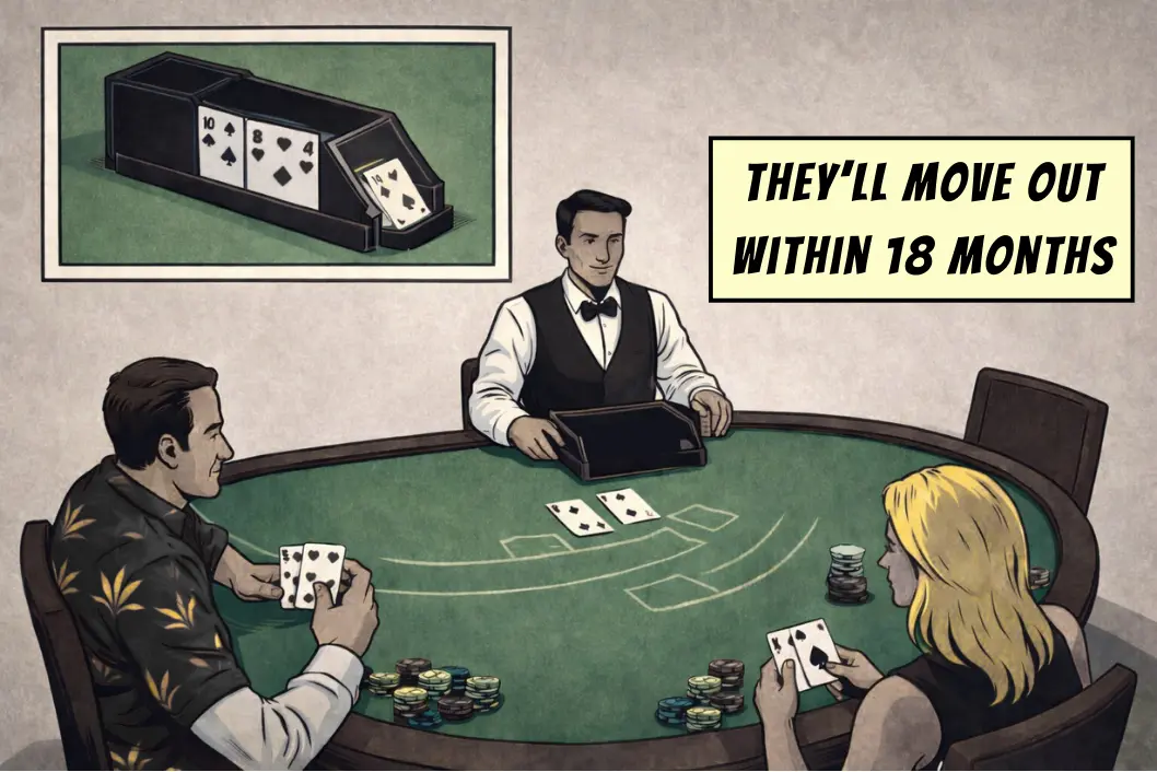
There's a useful analogy here to blackjack.
In blackjack, you can't control which cards get dealt. You can't predict the next card with certainty. But you can count the cards already played to understand what remains in the deck—and that changes your odds dramatically.
- When the deck is rich in high cards, you bet bigger
- When it's rich in low cards, you bet smaller
- The count doesn't give you certainty, but it does tilt probability in your favor
Rent-controlled buildings work the same way.
You can't control when tenants leave. But the current tenancies tell you the odds. Each tenant's position versus market rent determines their likelihood of moving—and that information is sitting right there in the rent roll. The current rent roll is your card count.
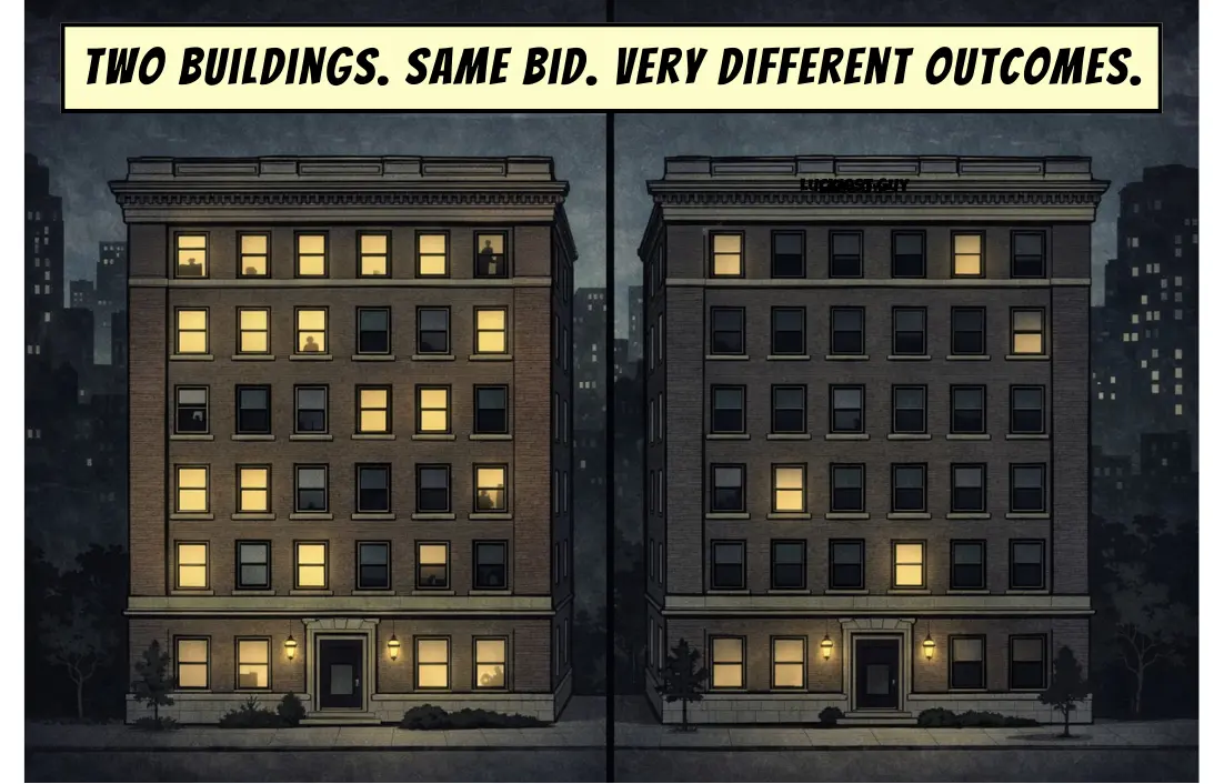
Two buildings, one illusion
Here's where this matters for acquisition decisions:
Imagine two identical buildings. Same location. Same quality. Same unit mix. Both show 8% embedded rent today. Traditional models value them identically. But look closer at their rent rolls:
Building A: Most tenants clustered around 5-10% below market. A few units at market rent and no units deeply discounted. The embedded rent is distributed across many units, each with a small gap.
Building B: Wide distribution. Half the units at or above market. The other half 15-25% below market. Same total embedded rent, but it's concentrated in fewer units with larger discounts.
Traditional underwriting sees two buildings with 8% upside, but in reality, these buildings will perform completely differently over your hold period.
The two buildings might appear to provide identical IRRs, but Building B will likely perform much worse.
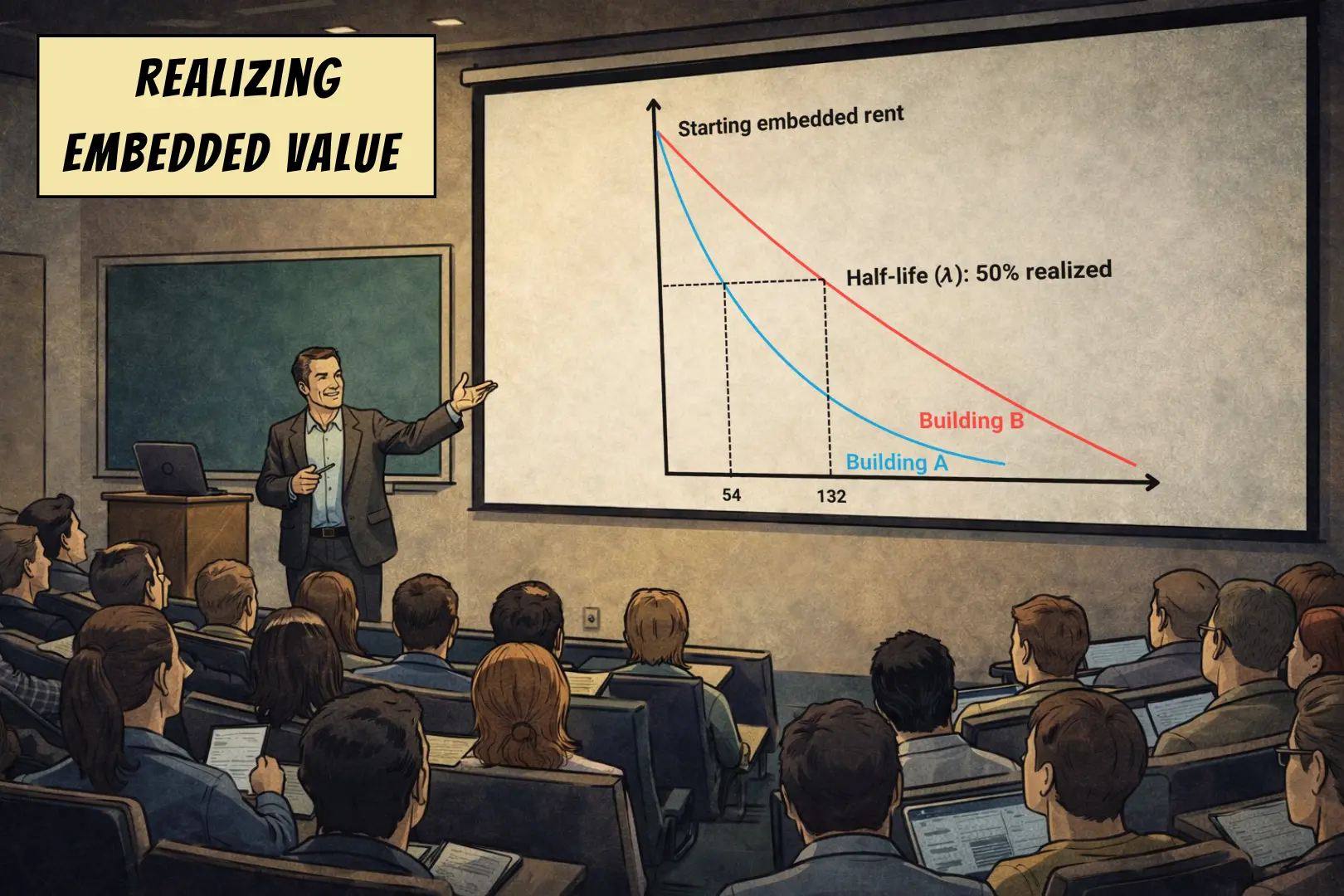
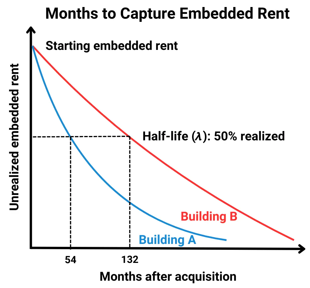
The half-life question
The better question isn't "How much embedded rent exists?"
It's: "How long until half of this embedded rent gets realized?"
This is Embedded Rent Half-Life—the time it takes for 50% of the upside to materialize through natural tenant turnover.

- Building A (many small discounts): Embedded Rent Half-Life of 54 months
- Building B (few large discounts): Embedded Rent Half-Life of 132 months
If your hold period is 5 years (60 months):
- Building A: You'll capture just over half of the embedded rent
- Building B: You'll be lucky to capture a quarter of the embedded rent
Same embedded rent today. Radically different outcomes. Oddly, both buildings might have the same turnover rates–the problem being that in Building B, it's your most valuable tenants, the ones paying the most rent, that are constantly churning.
And here's what makes this dangerous: Building B still looks attractive. You'll capture real value. The NOI will grow. Your model won't break spectacularly—it will just be wrong about timing. You'll pay for value that future owners–not you–will unlock.
The acquisition decision, reframed
The traditional question is: "Does this building have enough embedded rent to justify the price?"
The better question is: "Will this embedded rent materialize in time to generate my target return?"
You can't answer that by applying an average turnover rate. You need to understand the distribution—which tenants are likely to move, and when.
Two buildings with identical embedded rent can have completely different half-lives. That difference is worth millions in a competitive bid situation.
Reading the count
The answer exists in your portfolio data.
Your historical leases show exactly how tenants in your buildings behave at different rent positions. How long they stay when they're at market versus 5% below market versus 15% below market. How their tenure changes as their discount shrinks or grows over time.
That data reveals your Turnover Curves—the relationship between a tenant's rent position and how long they actually stay.
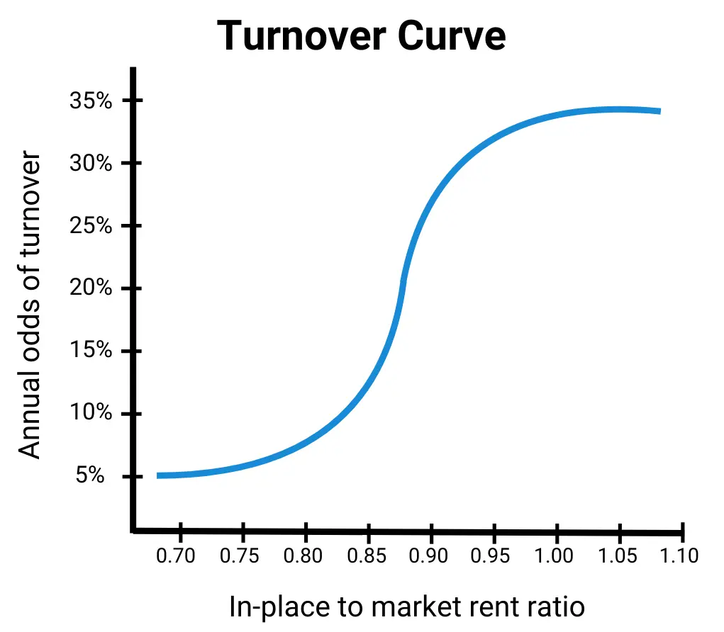
Turnover Curves are the equivalent of knowing the card count.
Some markets show dramatic tenure differences based on rent position. In others, the difference is minimal. Your one-bedrooms in Toronto highrises might follow one curve. Your two-bedrooms in Montreal mid-rises might follow another. The more units of each type you have, the clearer the pattern becomes.
This is a data advantage.
If you own 2,000 units across Ontario, you can predict tenant behavior in buildings you don't yet own—as long as they're in similar markets with similar unit types. Your existing portfolio tells you what's likely to happen in acquisition targets.
Competitors without that data are still guessing while you've been counting cards. You can count cards. Each property you look at is a hand of blackjack and by knowing the card count, you can bet big when the odds are in your favor and avoid losing money when they are not. This is why casinos refuse service to people counting cards–it's too big of an advantage.
But here's what doesn't work: industry averages, generic assumptions, or rules of thumb. Turnover curves are market-specific, building-type-specific, and unit-type-specific. They change over time as regulations and market conditions shift.
The only reliable way to derive them is from your own portfolio data—and that requires enough units to see clear patterns.
The bidding advantage
Think about what this means in a competitive acquisition process.
You and three competitors are bidding on the same building. All four of you see 10% embedded rent. All four of you run DCF models with 20% turnover assumptions. All four of you calculate similar IRRs.
But you've derived turnover curves from your portfolio. You can see that this specific rent roll—with its particular distribution of tenant positions—has a 4.5-year half-life. Most of the embedded rent will materialize within your hold period.
Your competitors are underwriting it with an 8-year half-life without realizing it. They're being conservative because they don't trust their own assumptions.
You can bid higher and still hit your return targets. You win the deal.
Or consider the opposite: A building with 10% embedded rent comes to market. Everyone gets excited. Your competitors start penciling aggressive bids.
But your curves tell you this rent roll has an 11-year half-life. The embedded rent is real, but it's locked deep—concentrated in units with 20%+ discounts where tenants will sit for a decade. You'll barely capture any of it in a 5-year hold.
You pass. Your competitors overpay.
This is the difference between counting cards and playing blind.
It's not just about making better decisions on individual buildings—it's about systematically winning the deals you should win and avoiding the ones you shouldn't. Over a dozen acquisitions, that edge compounds.
The information you need is already in your data. The current rent roll isn't just a snapshot of today's income—it's a predictor of which units will turn over and when.
You're sitting at a blackjack table. The count is sitting right in front of you. Every other bidder is playing blind.
The question isn't whether embedded rent exists — it's whether it belongs to you or the next buyer.
ReturnSuite provides analytical tools to Principal Owners looking to make better acquisition and operational decisions in complex real estate systems—like using turnover curves to optimize lease-up decisions in rent-controlled markets.